
 Download:


-
The infection rate of schistosomiasis in China now is at the lowest level in history, and the source of infection has been effectively controlled. However, the area of Oncomelania hupensis(O. hupensis), the only intermediate host of the genus Schistosoma, has been maintained at about 3.5 billion m2. Affected by the changes in climate, environment, and human activities, newly emerging and reemergent habitats of O. hupensis often occur, which makes early warning of O. hupensis become particularly important. Based on the surveillance data of O. hupensis (1), a niche model was used to predict the distribution of O. hupensis. The results indicated that the distribution of O. hupensis had concentrated, becoming primarily distributed in the middle and lower reaches of the Yangtze River, Dongting Lake, and Poyang Lake. Forecasting the distribution of O. hupensis is conducive to improving the ability of early warning of potential transmission risk and the elimination of schistosomiasis.
Schistosomiasis, a widespread zoonotic disease transmitted by the parasite of Schistosoma japonicum(S. japonicum), is considered as one of the most severe public health threats in China. O. hupensis is the only intermediate host of S. japonica and plays a key role in schistosomiasis transmission, whose geographical distribution reflects the area at risk of schistosomiasis transmission. According to the National Schistosomiasis Reporting System, the reported snail distribution has been maintained at about 3.5 billion square meters since 2004, and the occurrence and recurrence of snails have been reported in many areas (2). In 2016 and 2020, the Yangtze River Basin and its southern region suffered from 2 catastrophic floods. After the floods, suitable areas for snail breeding were formed, which increased the potential scope and degree of schistosomiasis distribution (3).
The environment with newly emerging and reemergent snail habitats from the national schistosomiasis surveillance sites from 2015 to 2019 were selected as the sample points, and 14 climatic, geographical, and socioeconomic factors (Supplementary Table S1) influencing O. hupensis distribution were collected as predictors. Spatial scanning based on Poisson model in SaTScan (version 9.6) was used to analyze the aggregation of newly emerging and reemergent habitats of O. hupensis. A total of 10 common niche models (Supplementary Table S2) provided in biomod2 platform (version 3.4.6) in R software (version 3.6.1; RStudio Inc; the USA) were used to construct single models, and the area under the curve (AUC) and true skill statistics (TSS) were used as the indicators of model screening, which were threshold-related indicators and threshold independent indicators commonly used to evaluate model accuracy. Single models were selected according to the criteria of AUC >0.90 and TSS >0.85. The weights were determined according to the TSS of the results of different algorithms, and the combined niche model was calculated by the weighted average method. The judgment threshold is defined as the minimum existence threshold, and the distribution probability from 0.00 to the minimum existence threshold is taken as the no-risk area, the minimum existence threshold to 0.70 is the low-risk area, 0.70 to 0.90 is the medium-risk area, and the greater than 0.9 is the high-risk area ( 4).
Category Variable name Source Climate factor ≥0 °C annual accumulated temperature http://www.resdc.cn ≥10 °C annual accumulated temperature Aridity Index of Moisture Average annual precipitation Average annual temperature Geographical factor Landform http://www.geodata.cn Land use Elevation http://www.resdc.cn Sand Silt Clay Socioeconomic factor Gross domestic product http://www.resdc.cn Density of population Table S1. Summary of environment variables used in the study.
Classification Model name Environmental envelope theory Surface range envelope Statistical regression algorithm Generalized linear model Generalized additive model Multivariate adaptive regression spline Statistical classification algorithm Generalized boosted model Classification tree analysis Flexible discriminant analysis Machine learning algorithm Artificial neural networks Random forest Maximum entropy Table S2. Summary of niche models used in the study.
According to the results of SaTScan scanning, six cluster areas in newly emerging and reemergent habitats of O. hupensis were detected, which were primarily distributed in the northwest region of Yunnan Province, the central part of Sichuan Province, and the junction of Jiangsu Province, Anhui Province, and Zhejiang Province (Figure 1). The prediction performance of 10 niche models was statistically significant through Kruskal-Wallis H test (AUC, H=24.720, P<0.05; TSS, H=29.372,P<0.05), and random forest (AUC=0.973, TSS=0.998) demonstrated the best prediction performance (Supplementary Table S3). Taken together, the importance of environmental variables in each model is different, of which the average annual rainfall and average annual temperature had more impacts (Supplementary Table S4). The current distribution of O. hupensis predicted by combination model indicated that the potential distribution areas of O. hupensis were mainly concentrated in the middle and lower reaches of the Yangtze River (Figure 2). These areas were also locally concentrated in the central part of Sichuan Province and scattered in the northwest part of Yunnan Province (Figure 2). Based on the predicted results of the niche model, the potential distribution area of O. hupensis accounted for 22.92% of the total area in China, and the distribution area can be categorized into areas of low-distribution (8.74%), medium-distribution (7.99%), and high-distribution (6.19%).
 Figure 1.
Ranges of newly emerging and reemergent habitats of Oncomelania hupensis and cluster area in schistosomiasis endemic areas, 2015−2019.
Model TSS (mean ± SD) AUC (mean ± SD) GLM 0.868 ± 0.057 0.947 ± 0.042 GBM 0.950 ± 0.007 0.996 ± 0.001 GAM 0.926 ± 0.008 0.990 ± 0.001 CTA 0.945 ± 0.009 0.980 ± 0.005 ANN 0.813 ± 0.056 0.930 ± 0.032 SRE 0.651 ± 0.018 0.825 ± 0.008 MARS 0.846 ± 0.251 0.946 ± 0.133 FDA 0.914 ± 0.015 0.983 ± 0.006 RF 0.973 ± 0.004 0.998 ± 0.001 MaxEnt 0.815 ± 0.023 0.915 ± 0.023 Abbreviation: TSS=True skill statistics; AUC=Area under the curve; SD=Standard deviation; GLM=Generalized linear model; GBM=Generalized boosted model; GAM=Generalized additive model; CTA=Classification tree analysis; ANN=Artificial neural networks; SRE=Surface range envelope; MARS=Multivariate adaptive regression spline; FDA=Flexible discriminant analysis; RF=Random forest; MaxEnt=Maximum entropy. Table S3. Performance evaluation indicators results of 10 niche models used in the study.
Model GLM GBM GAM CTA ANN SRE MARS FDA RF MaxEnt AAT 22.02 34.93 29.21 35.22 13.02 11.88 43.54 25.83 27.62 19.01 AAP 17.70 18.61 15.72 24.72 16.44 11.54 12.57 26.11 10.35 5.75 IM 18.45 9.73 8.24 0.34 31.16 10.03 17.78 15.69 4.75 9.11 LF 7.28 24.28 13.29 12.15 6.78 10.68 5.31 8.33 15.85 7.13 GDP 1.07 5.62 0.03 15.76 2.16 9.71 2.57 8.40 16.49 9.36 AR 6.32 1.22 5.53 0.21 11.17 9.17 5.71 2.92 0.90 11.02 EL 10.76 0.03 2.07 0.60 10.73 4.75 0.88 1.77 4.75 9.04 AAT0 8.61 0.48 5.56 2.53 0.53 6.39 2.79 6.08 10.29 9.18 DP 1.82 0.45 0.22 0.12 4.84 0.68 1.33 1.35 3.94 6.19 LD 0.51 1.54 10.25 5.36 0.61 8.82 3.93 1.42 1.42 1.35 Sand 0.81 1.81 4.66 2.49 0.39 6.88 0.90 0.80 2.23 1.30 AAT10 2.63 0.49 1.42 0.07 0.38 3.21 1.45 0.87 0.40 7.05 Silt 0.09 0.37 3.69 0.03 0.74 5.38 0.50 0.38 0.48 0.35 Clay 1.94 0.43 0.11 0.40 1.04 0.88 0.74 0.03 0.54 4.18 Abbreviation: AAT=Average annual temperature; AAP=Average annual precipitation; IM=Index of moisture; LF=Landform; GDP=Gross domestic product; AR=Aridity; EL=Elevation; DP=Density of population; LD=Land use; AAT0, ≥ 0 ℃ annual accumulated temperature; AAT10, ≥ 10 ℃ Annual accumulated temperature. GLM=Generalized linear model; GBM=Generalized boosted model; GAM=Generalized additive model; CTA=Classification tree analysis; ANN=Artificial neural networks; SRE=Surface range envelope; MARS=Multivariate adaptive regression spline; FDA=Flexible discriminant analysis; RF=Random forest; MaxEnt=Maximum entropy. Table S4. Importance percentage (%) of environmental variables of 10 niche models used in the study.
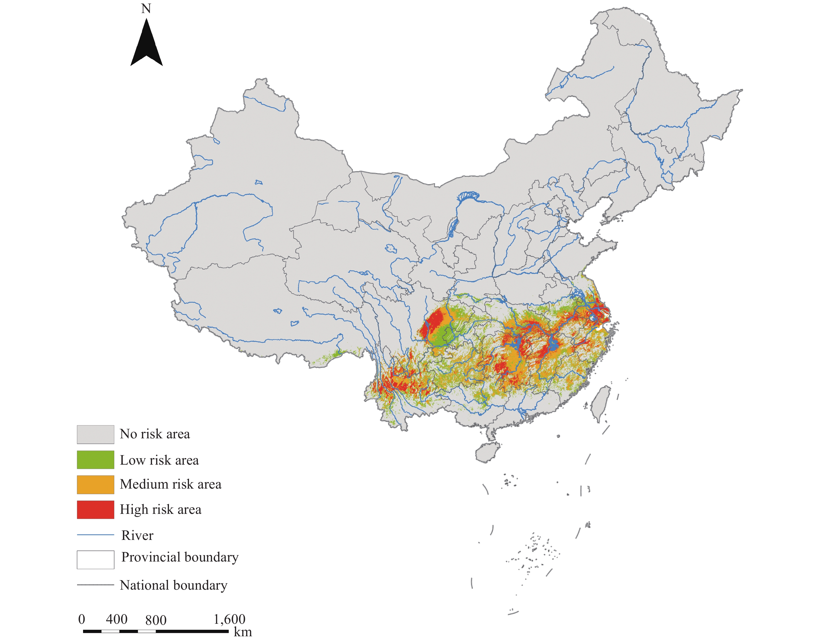 Figure 2.
Current distribution prediction map of Oncomelania hypensis in China based on combination model.
HTML
-
The results of this study indicated that the certain geographical aggregations in the potential high distribution areas of O. hupensis were primarily distributed in Poyang Lake area, Dongting Lake area, and the middle and the lower reaches of the Yangtze River. These areas maintain high water levels due to floods in summer and begin to recede in fall and winter. The seasonal periodic water-level changes lead the coastal beaches to form a wet meadow ecosystem, providing a suitable breeding place for O. hupensis (5). Due to fishing, grazing, farming, and other production and living reasons, residents were more likely to be exposed to snail environment and contaminated water (6). O. hupensis was distributed locally in the central part of Sichuan Province and scattered in the northwest part of Yunnan Province. Different from lake-marsh type snails distributed along the beach, the general law of the distribution of hilly snails is that they are distributed in the breeding environment of different topography with the water system from top to bottom. The migration and diffusion of Oncomelaniasnails are related to the size, distribution, velocity, and irrigation of water system. Affected by flood erosion, O. hupensis with higher terrain may spread with water flowing down the mountain, increasing the potential risk of schistosomiasis transmission (7).
Compared with the research of Liao et al. (8), this study used the latest snail survey data and combined the niche model to overcome the uncertainty brought by the single model. The high-risk areas of O. hupensis are basically consistent with the distribution patterns of schistosomiasis transmission in China (9). Compared with the risk distribution of schistosomiasis transmission assessed by Duan et al. (10), the high-risk areas predicted in this study covered a wider area, while the range of middle-areas and low-risk areas was lower than predicted and might be related to different sample points and predictors of two studies.
This study was subjected to some limitations. First, newly emerging and reemergent habitats outside the surveillance sites might have occurred, and this study did not take these sample points into account. Second, due to the unavailability of data, this study did not consider the impact of other human factors such as water conservancy projects, water supply reconstruction, and lavatories. In future research, more complete data of snail distribution are essential and can be accurately obtained through field investigation. More relevant variables from socioeconomic and environmental fields are necessary to be added to model training to improve the accuracy and effectiveness of the model prediction, promote the prediction results of potential snail distribution areas, and provide further technical support for the prevention, control, and monitoring of schistosomiasis.
Affected by production activities, natural disasters, water conservancy projects, climate change, and other factors, the abnormal spread of O. hupensis leads to the recurrence of schistosomiasis in some areas and even the spread to historically non-endemic areas. Historical experience suggests that there will be a relative peak in the area and the density of snails three years after flooding, which will increase the risk of repeated outbreaks of schistosomiasis and difficulty in schistosomiasis control (6). Although the national schistosomiasis control program in China has made great strides towards the interruption of transmission, the risk of schistosomiasis transmission still exists in some areas. To further consolidate the results of the national schistosomiasis control program and prevent rebound of schistosomiasis, taking comprehensive control strategies and measures in areas at risk of O. hupensis infestation is necessary.
Conflicts of interest: There are no conflicts of interest to declare.
| Citation: |

|