Methods and Applications: Optimization of Population-Level Testing, Contact Tracing, and Isolation in Emerging COVID-19 Outbreaks: a Mathematical Modeling Study — Tonghua City and Beijing Municipality, China, 2021–2022

The daily infection data were collected from the Beijing and Tonghua health commission websites. The population size was obtained from the local Statistics Bureau or government census data.

To evaluate the effectiveness of population-level testing (PLT) and contact tracing (CT) strategies, two transmission models were developed in this study. First, a transmission model incorporating PLT and CT was introduced to set up the context of modeling. Then, the model was extended to take age structure into account. Please see the Supplementary Materials for more details on this.

The probability of detecting COVID-19 cases under routine testing is a function of the sensitivity of PCR tests, the testing rate, and the particularized dynamics of the outbreak. To model the dynamic of an outbreak, an extended Susceptible-Exposed-Infectious-Removed (SEIR) model was developed. Please see the Supplementary Materials for more details on this.

A PLT strategy was one of the combinations: the time lag between the date of the first case identified and the date of the PLT launched (ranging anywhere from 1 to 7 days), population-level testing intervals (i.e. the time to complete 1 round of testing, including sample collection and reporting results, set to be either 2, 3, 4, 5, 7, or 10 days) and the break intervals between sequential rounds of testing (set to be either 0, 1, or 2 days) — which are often needed as a break for the testing staff. The total days considered to complete 1 round of testing was the testing interval plus the break interval. The outbreak duration divided by the total days needed to complete 1 round of testing was calculated as the rounds of PLT.

Resurgences of SARS-CoV-2 occurred in Tonghua (B.1.1 variant) in Jan-Feb of 2021, and Beijing (Omicron variant) in April-Jun of 2022. Once an index case was identified, CT was launched. To rapidly detect SARS-CoV-2 infections, the cities launched population-level PCR tests. To contain the transmission, Tonghua performed 3 rounds of testing — whereas Beijing conducted 26 rounds. After multiple rounds of PLT, there were no new cases reported, with the recurrence ultimately seeing 318 cases in Tonghua and 2,230 cases in Beijing.

A transmission-dynamic model without age structure (Figure 1) was fitted using the daily new infections identified from both PLT and CT in Tonghua. The model assumed all infected individuals were identified either from CT or PLT, and were then quarantined and removed from the transmission chain.

Figure 1. 

Simplified illustration of models. (A) A schematic of coronavirus disease 2019 (COVID-19) outbreak control and surveillance in China. (B) The transmission-dynamic model.

Note: In the transmission dynamic model, the following compartments are considered: susceptible (S), exposed (E), infectious pre-symptomatic (P), infectious asymptomatic (A), infectious symptomatic (I), and recovered (R). Compartments for infections identified through population-level testing (T) or contact tracing (C) as well as healthy individuals in quarantine (Q) are also included. The infections in T and C are isolated. β_A, β_P, β_I are the transmission rates for infectious asymptomatic, pre-symptomatic, and symptomatic cases, respectively. p_a is the proportion of asymptomatic cases.1/γ_E is the latent period. 1/γ_P is the pre-symptomatic period for symptomatic cases. 1/γ_A and 1/γ_I are the time to recover for asymptomatic and symptomatic cases, respectively. τ represents the rate of population-level PCR tests. 1/q is the time for quarantine. ω is the decay rate of antibodies for the individual in R. For further details, please refer to the methods section.

Abbreviation: PLT=population-level testing; CT=contact tracing.

Using the estimated parameters for Tonghua, this study evaluated the effectiveness of different PLT strategies in the containment of COVID-19 flare-ups. The required number of rounds of testing increased with the decreasing success fraction of CT if the testing interval remained unchanged (Figure 2A). If the success fraction of tracing remained unchanged, decreasing the testing interval not only reduced the necessary number of testing rounds, but also shortened the outbreak duration (Figure 2B).

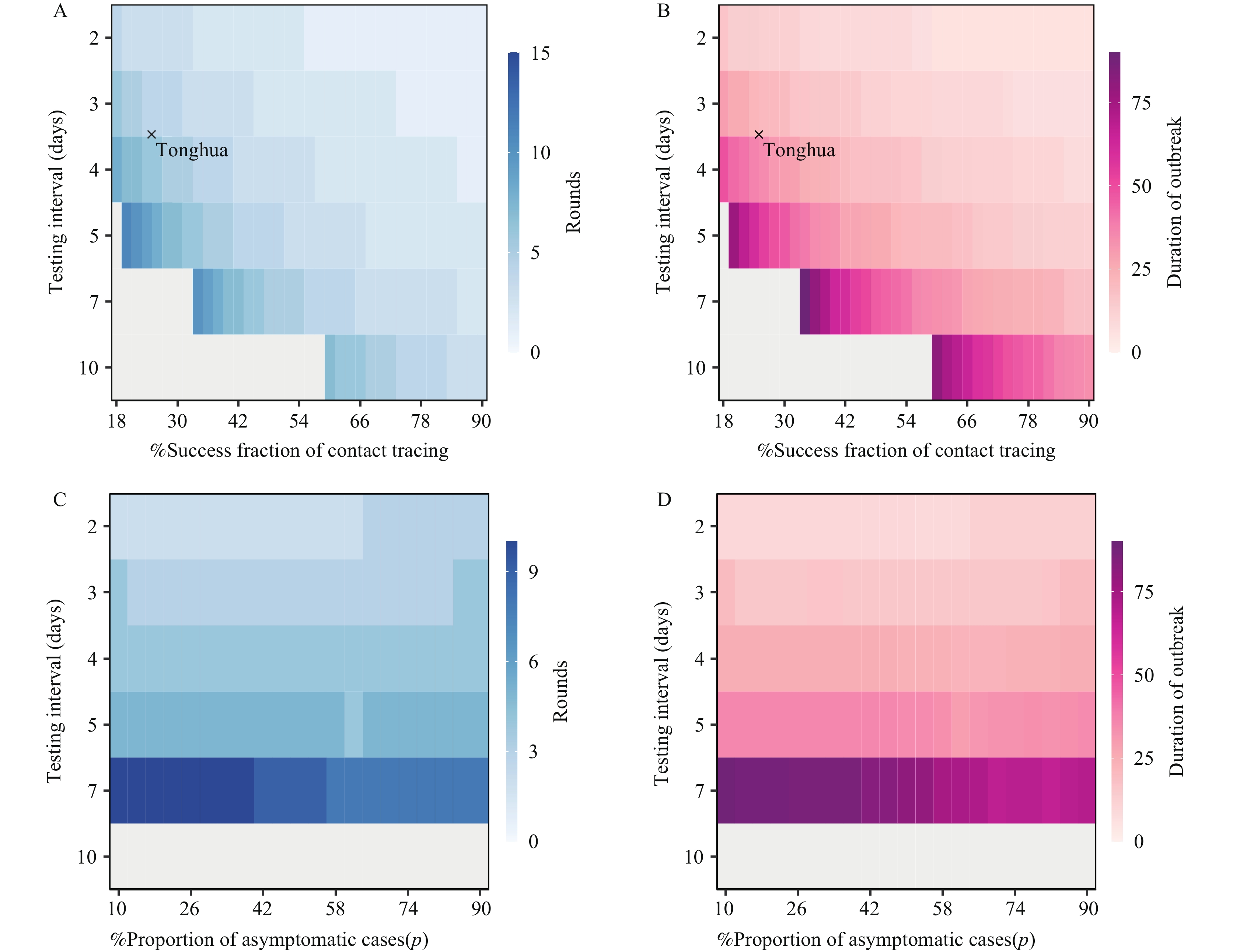Figure 2. 

The effects of PLT strategies, CT, and asymptomatic proportion on mitigation of COVID-19 flare-up outbreaks in Tonghua City. (A) The number of rounds of tests required to contain transmission for the B.1.1 lineage. (B) The corresponding outbreak duration (days) in (A). (C) The effects of the proportion of asymptomatic cases on the required rounds of testing for the B.1.1 lineage. (D) The corresponding duration of flare-up outbreaks in (C).

Note: For panels A–D, the break interval is 2 days and the time lag is 3 days. For panel B, columns correspond to the success fraction of CT: the fraction of contacts that were successfully traced (κ). Rows correspond to the number of days needed to complete a population-level round of testing. For panels C–D, the success fraction of contact tracing is set to 0.35. Grey areas represent parameter combinations by which outbreaks would not be controlled. This study defined that the outbreak was under control if the daily new infections were zero for 2 successive days. The number of rounds of PLT was calculated as the days to control the outbreak divided by the total days to complete 1 round of testing.

Abbreviation: COVID-19=coronavirus disease 2019; PLT=population-level testing; CT=contact tracing.

Our analyses show that the time lag, the testing interval, and the break interval have important effects on outbreak control. For a given testing interval, longer time lags necessitate more rounds of testing and result in longer durations of flare-ups (Figure 3A and D). Similar issues are predicted for increasing testing intervals if the time lag is fixed (Figure 3).

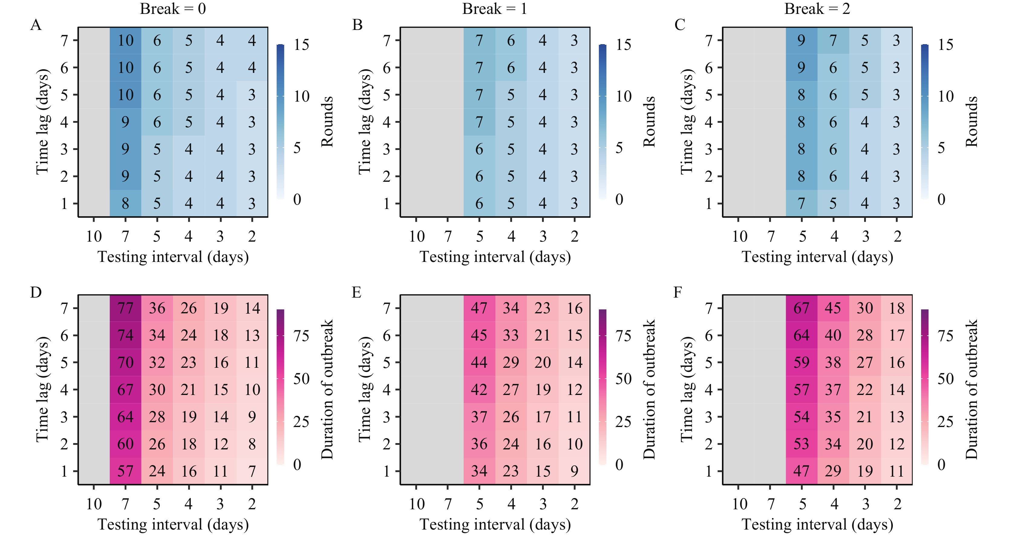Figure 3. 

The effects of time lag, testing interval, and break interval on mitigation of B.1.1 outbreaks in Tonghua. (A) Rounds of PLT required to contain transmission at Break interval=0. (B) Rounds of PLT required to contain transmission at Break interval=1. (C) Rounds of PLT required to contain transmission at Break interval=2. (D) The corresponding outbreak duration (days) in (A). (E) The corresponding outbreak duration (days) in (B). (F) The corresponding outbreak duration (days) in (C).

Note: In panels A–C, the number in each cell represents the rounds of PLT needed to control the outbreak. The success fraction of CT is set to 26% for (A) to (F). Rows correspond to the time lag between the date of the first case identified and the date of launching PLT. Columns correspond to the population-level testing interval. The break interval represents the break time between 2 sequential PLTs. The total time to complete 1 round of testing is the testing interval plus the break interval. The grey represents the PLT strategy by which the outbreak would not be sustained.

Abbreviation: PLT=population-level testing; CT=contact tracing.

We then extended the previous model to include age structure using the Omicron infection data from Beijing.

Based on the estimated parameters for Beijing, the effects of different testing rates for different age groups were explored (Figure 4). Overall, the simulation showed that the Omicron resurgence in a city could be controlled by multiple rounds of PLT. However, variations in the average number of tests needed per individual under different testing strategies were observed (Figure 4). The 21–60 age group has an important role in COVID-19 transmissions (Figure 4B). The modeling results demonstrate that, taking the average number of tests per individual as a benchmark, an appropriate frequency of tests for all age groups would be the best testing strategy to combat Omicron outbreaks.

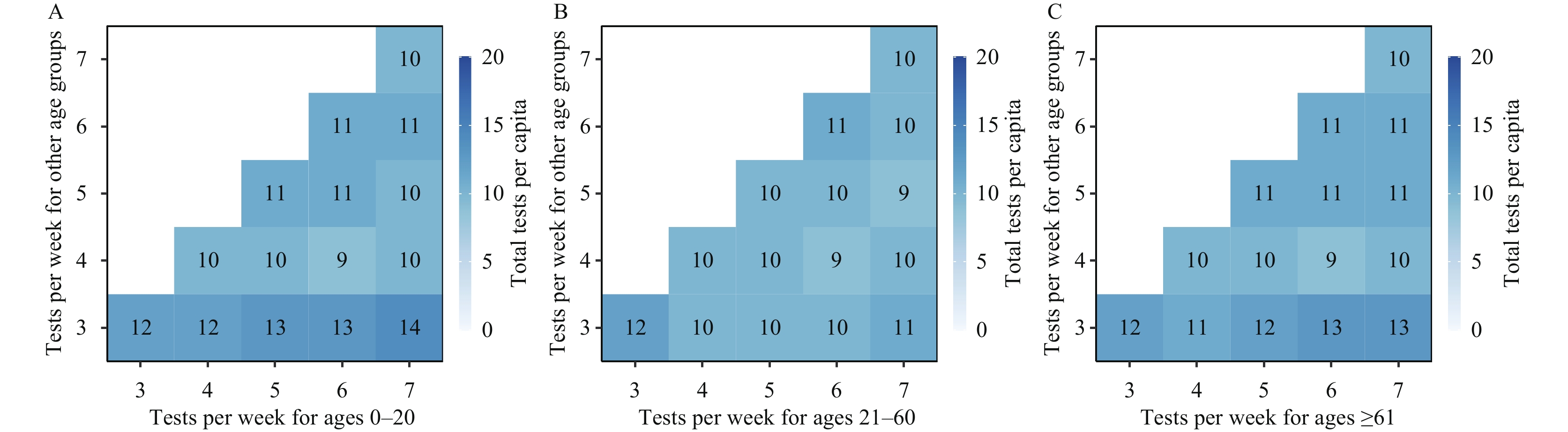Figure 4. 

The needed total tests per capita to control Omicron wave under different testing strategies in Beijing Municipality. (A) The testing frequency for ages 0–20 years. (B) The testing frequency for ages 21–60 years. (C) The testing frequency for ages ≥61.

Note: The testing frequency for other age groups is smaller or equal to that for ages 0–20. Each cell represents the total tests per capita.

Routine testing is critical for COVID-19 surveillance. The routine testing rate and the targeted population for testing have impacts on the time it takes to detect a COVID-19 flare-up. We developed a model to estimate the cumulative distribution of time needed to detect COVID-19 cases since an undetected SARS-CoV-2 infection was imported. If routine testing is applied to all age groups, there is a 90% probability of detecting COVID-19 cases within 3 days using daily testing. Otherwise, it takes 7 days to detect COVID-19 cases with a 90% probability level under biweekly testing schemas (Figure 5A). If routine testing is applied to the 0–20 and ≥61 age groups, respectively, a longer delay to detect COVID-19 cases is observed (Figure 5B and 5D). However, the cumulative distribution of time needed to identify COVID-19 cases when testing the 21–60 age group is similar to that when testing all age groups (Figure 5C). This indicates that routine testing applied to the 21–60 age group for COVID-19 surveillance can achieve similar performance to that applied to all populations.

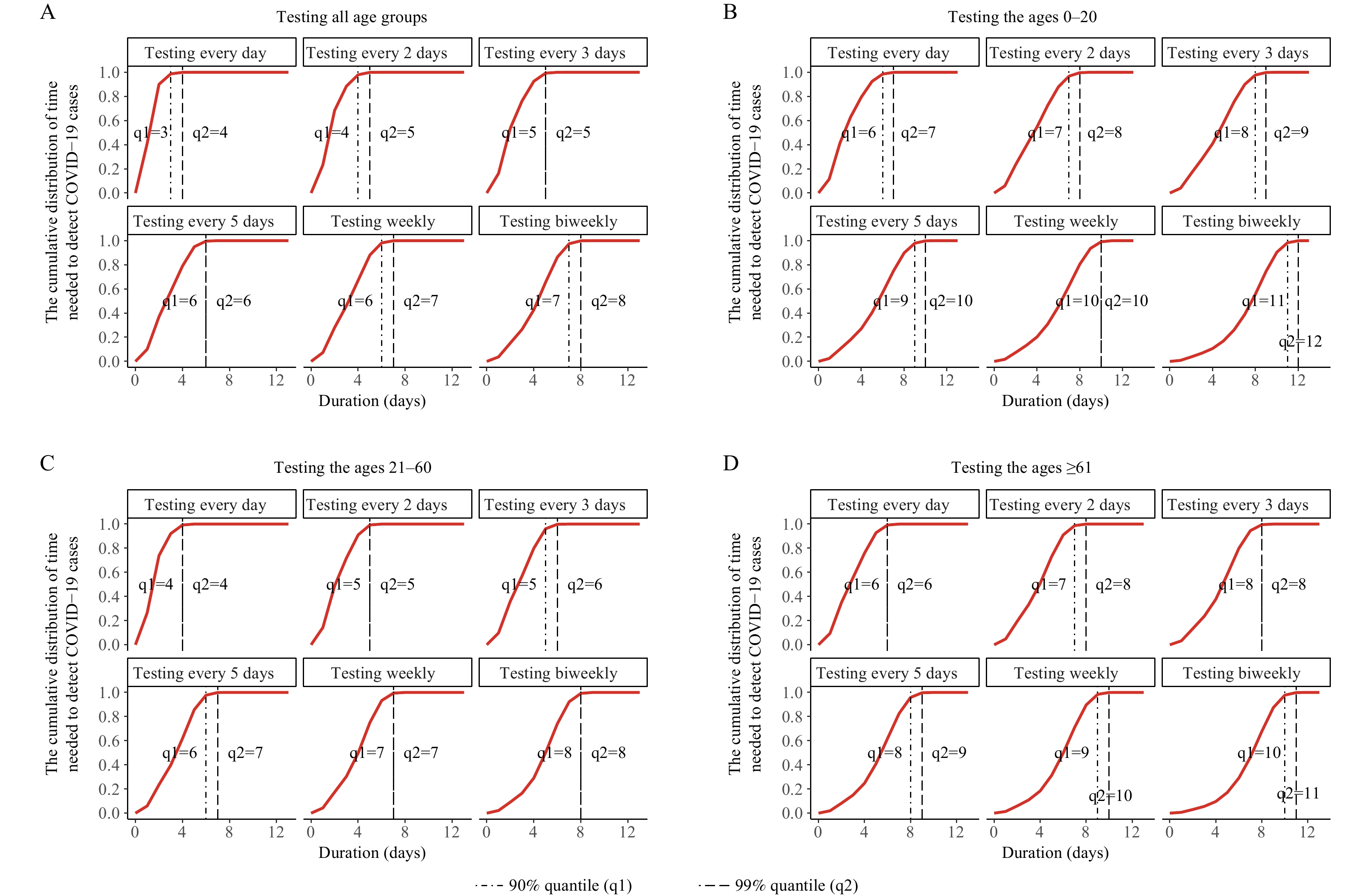Figure 5. 

The cumulative distribution of time (days) needed to detect coronavirus disease 2019 (COVID-19) cases under different routine testing strategies in Beijing for surveillance. (A) Testing all age groups. (B) Testing the ages 0–20. (C) Testing the ages 21–60. (D) Testing those aged ≥61.

Note: This study assumes that the first imported case was under exposed status and no reported SARS-CoV-2 infections occurred before the imported case. The duration is defined as the time interval from the date of importation of a COVID-19 case to the date of detecting at least 1 COVID-19 case by routine testing.

Using the data from SARS-CoV-2 flare-up outbreaks, this study evaluated the effects of PLT and CT on curbing COVID-19 resurgences. It showed that different combinations of PLT and CT lead to dramatically different scenarios of control. Considering the cost of PLT, there is both an economic and public health benefit to launching testing as early as possible and shortening testing intervals.

Testing capacity may be a challenge for some cities. However, a certain level of testing should be guaranteed given the dramatically enlarged capacity of polymerase chain reaction (PCR) tests and the new rapid testing methods made available since the start of the pandemic (13). Although the sensitivity of rapid antigen testing is lower than PCR tests, recent studies found that test sensitivity is secondary to frequency and turnaround time for COVID-19 screening (14). In regions with constrained resources, optimal pooled testing strategies may be employed (15).

The Omicron variant poses a great challenge for COVID-19 control. This study found that Omicron outbreaks could be controlled using multiple rounds of PLT. If new variants with higher transmissibility emerge, more rounds of PLT and a higher success fraction of CT would be needed to contain the outbreak. The PLT strategy can also be optimized among different age groups if the average tests per individual is used as a benchmark. Considering the importation of COVID-19 cases, this study also evaluated time needed to detect COVID-19 cases under different routine testing rates and different targeted testing populations for surveillance. The results indicate that testing the 21–60 age group for COVID-19 can achieve similar performance to that of testing all populations.

There are a few limitations to this study. In this model, no spatial heterogeneity is assumed. In reality, populations living in residential areas with high-rise housing would be priority tested multiple times. Further, individuals in high-risk regions would be tested first. Therefore, the necessary rounds of PLT would be smaller than the prediction in this research. In addition, the model with the constancy of population size is formulated because no travel in and out is assumed. This assumption thus implies that there are no imported COVID-19 cases after the outbreak was detected. In reality, Omicron outbreak is harder to control compared to the B.1.1 variant. However, the results for these two variants based on our analysis cannot be compared directly because the parameters for them are quite different. Next, due to the insufficient surveillance of SARS-CoV-2, the reproduction number, proportion, and clinical and immunological profiles of asymptomatic infections are still not clear (16-17). More studies about the immunity profile (induced by primary infection and vaccines) and the protection of different vaccines against different lineages are needed to calibrate such calculations in the future. Finally, the age distribution of imported COVID-19 cases is assumed based on the age structure of Beijing. However, the deviation of imported COVID-19 cases from this assumption would have influences on the effectiveness of routine testing — especially for the different target testing populations.

In summary, our modeling analysis provides insights to local governments on what is necessary to control future COVID-19 resurgences in regards to population-level testing and contact tracing. Further investigation is required to understand whether the outcomes of frequent population-level testing can be replicated outside the context of China.

No conflicts of interest.

We would like to acknowledge the CDC staff and local health workers in China who helped us collect data and who will continue to work to contain COVID-19 in China.

This section will introduce the models applied to the coronavirus disease 2019 (COVID-19) data in Tonghua City and Beijing Municipality, China.

Basic notations and set-up: We developed a transmission-dynamic model that incorporated the asymptomatic and symptomatic cases. Specifically, we considered susceptible (S), exposed (E), pre-symptomatic (P), infectious asymptomatic (A), infectious symptomatic (I), and recovered (R) individuals (see the model illustration in Figure 1). Control measures [population-level polymerase chain reaction (PCR) testing and contact tracing] were implemented, and the infected individuals were identified through either population-level testing (PLT) (T) or contact tracing (CT) (C). Therefore, they would be quarantined and exit the transmission chain. Healthy individuals may also be traced and quarantined (Q). Although the contacts detected by CT were large, they account for quite a small proportion of the overall population given the millions of people in Tonghua. The proportion of susceptible persons didn’t change a lot. 0 daily infections for 2 successive days was used as an index of a controlled flare-up. In this study, 1 round of PLT is defined as everyone tested 1 time in a population. The rounds of PLT needed to control resurgences was quantified.

Population-level testing and contact tracing in the model: Let τ (the proportion of population tested per day) represent the testing rate for a city. To simplify the model, the spatial heterogeneity of testing was not included. Further, the tracing and quarantining of secondary contacts were not modeled for simplicity. Due to the detailed epidemiological investigations available to learn from, onwards infections could be identified relatively effectively from CT and PLT even in individuals without overt symptoms. Once an infection was identified, the contacts would be in different compartments at the time of tracing. Therefore, traced individuals are removed through different compartments (see the model illustration in Figure 1). To model the contact tracing in a detailed way, the contact tracing rate, the contact tracing precision (i.e. the proportion of traced contacts who were infected), and the probability that a contact traced through an infection from compartment i had progressed to compartment j at the time of tracing was formulated.

Considering that the sensitivity of PCR testing depends on the disease’s progress, the PCR test sensitivities for different compartments were included. Specifically, ${\pi _E},{\pi _A},{\pi _P},{\pi _I}$ represent the sensitivity of PCR tests for the individuals in compartments E, A, P and I, respectively. This study then modeled the CT like those in the study of Davin Lunz et al. (1) with extension. The contact tracing rate α_i for compartment $i,i \in \{ E,A,P,I\} $ is given by the testing rate τ, the sensitivity of PCR test, the fraction of contacts that were successfully traced κ, the contact number per day M, and the pre-defined CT time window (L days), which is ${\alpha _i} = {\pi _i}\tau \kappa LM$. κ represents the strictness and capacity of CT in a city. L depends on the specific infectious disease. The contact tracing precision ${\theta _i}$ for the primary cases from compartment i is defined as the proportion of traced contacts through compartment i that were infected. It is related to the average transmission rate and the proportion of susceptible persons in the population, which is $ {\theta }_{i}=S{\widehat{\beta }}_{i}/(N\times M) $. N is the population size. For compartments A and P, $ {\widehat{\beta }}_{A}={\beta }_{A} $ and $ {\widehat{\beta }}_{P}={\beta }_{P} $. For compartment I, the average transmission rate is ${\widehat{\beta }}_{I}=\dfrac{{\beta }_{P}({\gamma }_{P}+\tau {\pi }_{P}{)}^{-1}+{\beta }_{I}({\gamma }_{I}+\tau {\pi }_{I}{)}^{-1}}{({\gamma }_{P}+\tau {\pi }_{P}{)}^{-1}+({\gamma }_{I}+\tau {\pi }_{I}{)}^{-1}}$. ${\beta _i}$ is the transmission rate for an individual in compartment i. Note that the individuals in E are not infectious and the contact precision for compartment E is 0. The contacts who were traced through infections in compartment i are removed at the rate of ${\alpha _i}{\theta _i}i$ and removed from compartment j with the proportion of ${p_{ij}}$, where $\sum\nolimits_{j \in \left\{ {E,A,P,I} \right\}} {{p_{ij}}} = 1$. Note that ${p_{ij}}$ depends on dynamic of COVID-19. Note that the contacts traced through the individuals in compartment i may be either not infected, or were infected by someone else rather than the identified cases. Therefore, they are removed at the rate ${\alpha _i}(1{\text{ - }}{\theta _i})i$. The full set of equations representing the transmission is given by

where

In this study,${p_a}$is the proportion of asymptomatic cases. 1/γ_E is the latent period. 1/γ_P is the pre-symptomatic period for symptomatic cases. 1/γ_A and 1/γ_I are the time to recover for asymptomatic and symptomatic cases, respectively. ${\beta _A},\;{\beta _P},\;{\beta _I}$ are the transmission rates for asymptomatic, pre-symptomatic, and symptomatic cases, respectively. This model takes ${\beta _A}$ for infectious asymptomatic individuals to be ${\lambda _1}{\beta _I}$ and ${\beta _P}$ for pre-symptomatic individuals to be ${\lambda _2}{\beta _I}$ similar to the setting of (2). Due to other detailed epidemiological investigations, onwards infections could be identified relatively effectively from CT even in individuals without overt symptoms. In the model, traced individuals are tracked through different compartments. Similar to CT, the infections can also be identified through different compartments by population-level PCR tests, regardless of presence or absence of symptoms. For the individuals in R, they will enter the state of S due to the decay of antibodies at a rate of $\omega $. It is set to be 0 unless otherwise stated. The quantities α_i, ${\theta _i}$ depends on the disease dynamic, ${\beta _I}$ and κ. For ${p_{ij}}$, it also depends on the disease dynamic and the CT delay (${t_0}$) and can be derived from the model. Please refer to the following sections for more details about ${p_{ij}}$. According to the next generation matrix, ${R_0} = {p_a}\dfrac{{{\beta _A}}}{{{\gamma _A}}} + (1 - {p_a})\dfrac{{{\beta _P}}}{{{\gamma _P}}} + (1 - {p_a})\dfrac{{{\beta _I}}}{{{\gamma _I}}}$. $ {\beta _n} $ is used to represent the reduced percentage of transmission rates due to other NPIs (for example, wearing face masks and following social distancing guidelines). Therefore, the actual transmission rate for symptomatic cases would be ${\beta _I}(1 - {\beta _n})$. The unknown parameters for this model are the reduced percentage of transmission rate (${\beta _n}$), the fraction of contacts that were successfully traced (κ), and the initial values for A, P, I, and E.

The model fitting: This study has two sets of observations: the daily new infections identified from CT and the daily new infections identified from PLT. It models the number of daily new infections identified by CT and the number of new infections identified by PLT as a random variable following Poisson distribution with expectation $\lambda _t^C$ and $\lambda _t^T$, respectively. Specifically,

${\alpha _I}{\theta _I}I(t) + {\alpha _P}{\theta _P}P(t) + {\alpha _A}{\theta _A}A(t)$ represents the infected contacts traced through infections in compartments A, P and I. $\mu \dfrac{{E(t) + A(t) + P(t) + I(t)}}{N}$ represents the traced contacts who were infected by someone else rather than the identified cases. Therefore, $\lambda _t^C$ is the mean of daily infections identified by CT. τ is the proportion of population tested per day and $\lambda _t^T$ is the mean of daily infections identified by PLT. This study fitted the model to 2 sets of observations with a 3-day rolling mean. Model fitting was performed using the Metropolis–Hastings Markov chain Monte Carlo (MCMC) algorithm with the MATLAB (version R2020a) toolbox DRAM (Delayed Rejection Adaptive Metropolis). 100,000 iterations were set for burn-in. After that, another 100,000 iterations were performed.

The calculation of $p_{ij}^g$: This section calculates the probability that a contact who was traced through an infection in compartment i has progressed to compartment j at the time of tracing, ${\text{i}} \in \left\{ {{\text{A, P, I}}} \right\}$, $ {\text{j}} \in \left\{ {{\text{E, A, P, I}}} \right\} $. The calculation process is similar to that in (1), but expanded to A, P and I compartments from different age groups. Note that the age group g should be omitted in the model without age structure. The full descriptions with age structure are given here. For readability, the details are described here. The transition probability is introduced

by assuming the individual progresses along a continuous-time Markov chain following the disease’s progress. With time-homogeneity, $ {P_{B,{\text{ }}{S_2}\left| {A,{\text{ }}{{\text{S}}_1}} \right.}}{\text{ = }}{P_{B,{\text{ }}{S_2} - {S_1}\left| {A,0} \right.}} = :{P_{B\left| A \right.}}({S_2} - {S_1}) $. Defining the time t=0 as the time of obtaining the positive PCR tests report for the tested case of age group g in compartment ${\text{i}} \in \left\{ {{\text{A, P, I}}} \right\}$, this study calculates the probability ($ p_{ij}^g $) that a contact traced through this case is in compartment $ {\text{j}} \in \left\{ {{\text{E, A, P, I}}} \right\} $ at $ {\text{t}} = {{\text{t}}_0} \geqslant 0 $. $ {t}_{0} $ represents the contact tracing delay. It is set to be 0 unless otherwise stated. Let $\mathbb{Q} $ be the probability density of an individual infecting a contact (given the individual tests positive at time t=0).

Similarly, there is

and

Above equations are continue-time. To be compatible with the model, $ v_{ij}^g $ will be calculated in discrete time way with step 1. At last, by normalizing, $p_{ij}^g = \dfrac{{v_{ij}^g}}{{\sum\limits_{j \in \left\{ {E,A,P,I} \right\}} {v_{ij}^g} }},i \in \left\{ {A,P,I} \right\}.$ $p_{ij}^g$ depends on the disease dynamic, testing rate (τ) and contact tracing delay ($ {t_0} $). Here we assume $ {t_0} = 0. $ $tL$ represents the entire period of COVID-19 and is set to 25 days.

Transition probability ${P_{B\left| A \right.}}$: In this section, we will calculate the transition probability. The derivation is same with that in (1). For readability, we write down the details. The transition probability is defined as

For the simplification, the transition rate from compartment K by $ \gamma _K^* $ is defined as $ \gamma _K^* = {\gamma _K} + \tau $. Note that $ \tau $ may be changing during the flare-up in reality. However, to facilitate the computation, we used the average of τ. Starting and finishing in the same compartment is

For the transition from J to K, the fraction of individuals who leave J that reach K as$ {q_{I \to K}} $$ . $ These are given by

Each transition requires a new integration and a reduction by the fraction of arrivals. So, we have

Similarly,

In this section, we extended above model and introduced the age-stratified population-level testing and contract tracing model. Specifically, we considered susceptible (S_b), exposed (E_b), pre-symptomatic (P_b), infectious asymptomatic (A_b), infectious symptomatic (I_b), recovered (R_b) individuals for age group b, b=1, …, G. The infected individuals in age group b would be identified through population-level testing (T_b) and contact tracing (C_b). Healthy individuals may also be traced and quarantined (Q_b). Next, we described how the contact tracing rate, the contact tracing precision and the probability that a contact traced through compartment i has progressed to compartment j at the time of tracing was formulated in details for age group b.

The contact tracing rate α_b is given by the testing rate τ (the proportion of population tested per day), the fraction of contacts that can be successfully traced $ \kappa $, the contact number per day M_bg with other age group g, and the pre-defined contact tracing time window (L days), which is $ {\alpha }_{b} $=$ {\pi }_{i}\tau \kappa L\left(\sum _{g=1}^{G}{M}_{bg}{i}_{g}\right) $. κ represents the strictness and capacity of contact tracing in a city. The contact tracing precision $ {\theta }_{bg}^{i} $ for the primary cases from compartment i in age group g contributing to age group b is defined as the proportion of traced contacts through compartment i of age group g were infected. It is related to the average transmission rate in age group g contributing to age group b and the proportion of susceptible in the population of age group b, which is $ {\theta }_{bg}^{i}={S}_{b}\widehat{{\mathrm{\beta }}_{bg}^{i}}/({N}_{b}\times {M}_{bg}) $. N_b is the population size for age group b. For compartment A and P, $ \widehat{{\beta }_{bg}^{A}}={{\phi }_{b}\beta }_{A}{M}_{bg} $ and $ \widehat{{\beta }_{bg}^{P}}={{\phi }_{b}\beta }_{P}{M}_{bg} $. For compartment I, the average transmission rate is $\widehat{{\beta }_{bg}^{I}}={\phi }_{b}\dfrac{{\beta }_{P}({\gamma }_{P}+{\pi }_{P}\tau {)}^{-1}+{\beta }_{I}({\gamma }_{I}+{\pi }_{I}\tau {)}^{-1}}{({\gamma }_{P}+{\pi }_{P}\tau {)}^{-1}+({\gamma }_{I}+{\pi }_{I}\tau {)}^{-1}}{M}_{bg}$. $ {\phi }_{b} $ is the susceptibility to infection for age group b and $ {\beta }_{i} $ is the probability of getting infected for each effective contact with individual in compartment i. Note that the individuals in E_b are not infectious and the contact precision for compartment E_b is 0. The contacts traced through compartment i are removed from age group b at the rate of $ {\pi }_{i}\tau \kappa L\left\{\sum _{g=1}^{G}{M}_{bg}{i}_{g}{\theta }_{bg}^{i}\right\} $ and removed from compartment j of age group b with the proportion of $ {p}_{ij}^{g} $, where $ {\sum }_{j\in \{E,A,P,I\}}{p}_{ij}^{g}=1 $. Note that $ {p}_{ij}^{g} $ depends on dynamic of COVID-19 in age group g. The full set of equations representing the transmission is given by

where

In our analysis, $ {p}_{a}^{b} $ is the proportion of asymptomatic cases for age group b. The quantities α_b, $ {\theta }_{bg}^{i} $ depend on the disease dynamic, $ {\beta }_{I} $ and κ. For $ {p}_{ij}^{g} $, it also depends on the disease dynamic and the contact tracing delay ($ {t}_{0} $) and can be derived from the model.

Similar to previous model, we modeled the number of daily new infections as a random variable following Poisson distribution with expectation $ {\lambda }_{t}^{C} $ and $ {\lambda }_{t}^{T} $ for contact tracing and population-level testing, respectively. Specifically,

We estimated the probability of detecting the first case $ Z $ for each day under routine testing since one SARS-CoV-2 infection was imported. Assuming the first detected case is found on the day $ t $, it means that no infections have been detected in the past $ t-1 $ days. $ Z={P}_{t}{\prod }_{k=1}^{t-1}(1-{P}_{k}) $. Hence, we first formulated the probability for detecting at least one case $ {P}_{t} $ for day t.

Assuming the total number of cases tested for day t is $ {B}_{t} $, We considered the number of cases tested positive as a binomial distribution with parameter $ {B}_{t} $ and $ {p}_{t} $. $ {p}_{t} $ represents the probability of success for each trial. Therefore, the probability for detecting at least one case for day t is $ {P}_{t}=1-{(1-{p}_{t})}^{{B}_{t}} $. The success probability $ {p}_{t} $ of having a positive PCR test for each tested case is a function of the testing sensitivity of PCR tests and the dynamics of outbreak. To simulate total number of cases tested $ {B}_{t} $, we also developed a transmission-dynamic model with age structure, which incorporated susceptible (S), exposed (E), pre-symptomatic (P), infectious asymptomatic (A), infectious symptomatic (I), recovered (R) compartment. It is important to note that no control measures were implemented to cut the transmission chain because of no reported cases. The full set of equations representing the transmission is given by

where

Considering that each tested case may be in any state of E, A, P, I, and the sensitivity of PCR testing in each status is different, we estimated daily average positive probability $ {p}_{t} $ weighted by the proportion of population for each status for day t. Specifically, we have

where $ {\tau }_{b} $ is the routine testing rate for age group b. We considered that the first imported infection is at the exposed (E) status and distributed among the age groups according to the age proportion of Beijing.　

Lunz D, Batt G, Ruess J. To quarantine, or not to quarantine: A theoretical framework for disease control via contact tracing. Epidemics 2021;34:100428. http://dx.doi.org/10.1016/j.epidem.2020.100428. Aleta A, Martín-Corral D, Piontti APY, Ajelli M, Litvinova M, Chinazzi M, et al. Modelling the impact of testing, contact tracing and household quarantine on second waves of COVID-19. Nat Hum Behav 2020;4(9):964 − 71. http://dx.doi.org/10.1038/s41562-020-0931-9.