Methods and Applications: High-Resolution Data on Human Behavior for Effective COVID-19 Policy-Making — Wuhan City, Hubei Province, China, January 1–February 29, 2020

The calibration of parameters is performed with the Python (version 3.6.0, Python Software Foundation, Wilmington, US) and the Python package PyMC (version 2.3.8). The data of COVID-19 cases (high-resolution) were sourced from the large epidemic network of China Electronics Technology Group Corporation (CETC), which was obtained indirectly from the front-line hospitals and disease control departments in Wuhan. Population mobility data was derived from China Mobile’s cell phone signaling records.

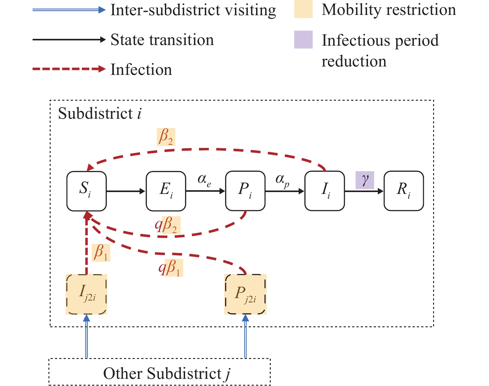
We adopt a metapopulation model to simulate the transmission of COVID-19 in Wuhan City. Supplementary Figure S1 shows the schematic diagram of the model. Our model treats each subdistrict as a metapopulation. For each subdistrict, the model divides the whole population into five compartments, i.e., the susceptible population $ S $, the exposed population $ E $, the pre-symptomatic infectious population $ P $, the infectious population $ I $, and the effectively removed population $ R $. Therefore, our model is named as a metapopulation Susceptible-Exposed-Presymptomatic-Infectious-Removal (SEPIR) model. The equations of transition relationships between the five populations are given as follows.

where $ i $ denotes the subdistrict index. The variables $ {S}_{i} $, $ {E}_{i} $, $ {P}_{i} $, $ {I}_{i} $ $ {R}_{i} $ denote the corresponding compartments’ population of the $ i $-th subdistrict. The parameter $ \beta $ is the transmission rate between susceptible and infectious populations. $ {\alpha }_{e} $ is the transition rate from the population $ E $ to $ P $, $ {\alpha }_{p} $ is the incidence rate, and $ \gamma $ is the removal rate.

The transition rate $ {\alpha }_{e} $ is set as the inverse of the average period between exposure and presymptomatic infectious (the incubation period minus 2.3 days), and the incidence rate $ {\alpha }_{p} $ is set as the inverse of the average presymptomatic infectious period (2.3 days). The removal rate $ \gamma $ was dynamically set as the inverse of the average duration from symptom onset to confirmation for every day. As shown in Supplementary Figure S2, this duration substantially reduces as a result of intervention policies.

In our model, we set the transmission rates $ \beta $ to be dynamic. Given a subdistrict $ i $, there were four transmission rates, namely $ {\beta }_{\mathrm{1,1}}^{i} $, $ {\beta }_{\mathrm{1,2}}^{i} $, $ {\beta }_{\mathrm{1,3}}^{i} $, $ {\beta }_{2}^{i} $. For any one of the four transmission rates, denoted as $ {\beta }_{*}^{i} $, we set it as $ {\beta }_{*}^{i}={\widehat{\beta }}_{*}^{i}\cdot {M}_{t}^{i} $ on the day t, where $ {\widehat{\beta }}_{*}^{i} $ was a basic transmission rate and $ {M}_{t}^{i} $ was the total volume of resident mobility in the subdistrict $ i $ on the day $ t $. The $ {M}_{t}^{i} $ was calculated as $ {M}_{t}^{i}=({\sum }_{ij}^{}{w}_{ijt}+{h}_{ijt}+{r}_{ijt})/{N}_{i} $, where $ {w}_{ijt} $ was the amount of inter-subdistrict mobility from subdistrict $ i $ to subdistrict $ j $ during the morning-peak (to-workplace) period, $ {h}_{ijt} $ was during the evening-peak (to-home) period, and $ {r}_{ijt} $ was during the off-peak period.

We derived the effective reproduction number $ {R}_{e} $ of the metapopulation SEPIR model by the next generation matrix. Suppose a model with $ m $ metapopulations, let $ x=({E}_{1},{E}_{2},\dots ,{E}_{m},{P}_{1},{P}_{2},\dots ,{P}_{m}, {I}_{1},{I}_{2},\dots ,{I}_{m})^{T} $ be the number of individuals for each infected compartments, ${u}_{i} = \dfrac{{S}_{i}}{{N}_{i}}{\beta }_{2,\;1}^{i}, {v}_{ji} = {\sum }_{h}^{}{\beta }_{1,h}^{i}\dfrac{{S}_{i}}{{N}_{i}}\dfrac{{T}_{hji}}{{N}_{j}}{c}_{j}.$ The detailed calculation process is shown in Supplementary Material.

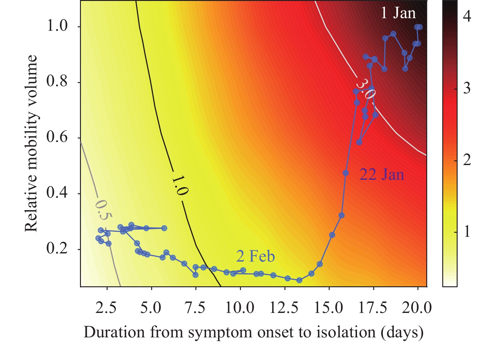
We adjusted the parameters of the calibrated model to estimate the effectiveness of different interventions and their interactions with the effective reproduction number $ {R}_{e} $. Using the calibrated model parameters on January 23, 2020 as the benchmark, we adjusted the resident mobility intensity, i.e., $ {w}_{ijt} $, $ {h}_{ijt} $, and $ {r}_{ijt} $, to simulate the effectiveness of the mobility restriction policy, as well as adjusted the average duration from symptom onset to isolation, i.e., $ 1/\gamma $, to simulate the effectiveness of the policies aiming to reduce the infectious period. We construct the contour plot of $ {R}_{e} $ in Figure 1A through traversing the relative resident mobility intensity and the average duration from symptom onset to isolation to generate corresponding effective reproduction numbers.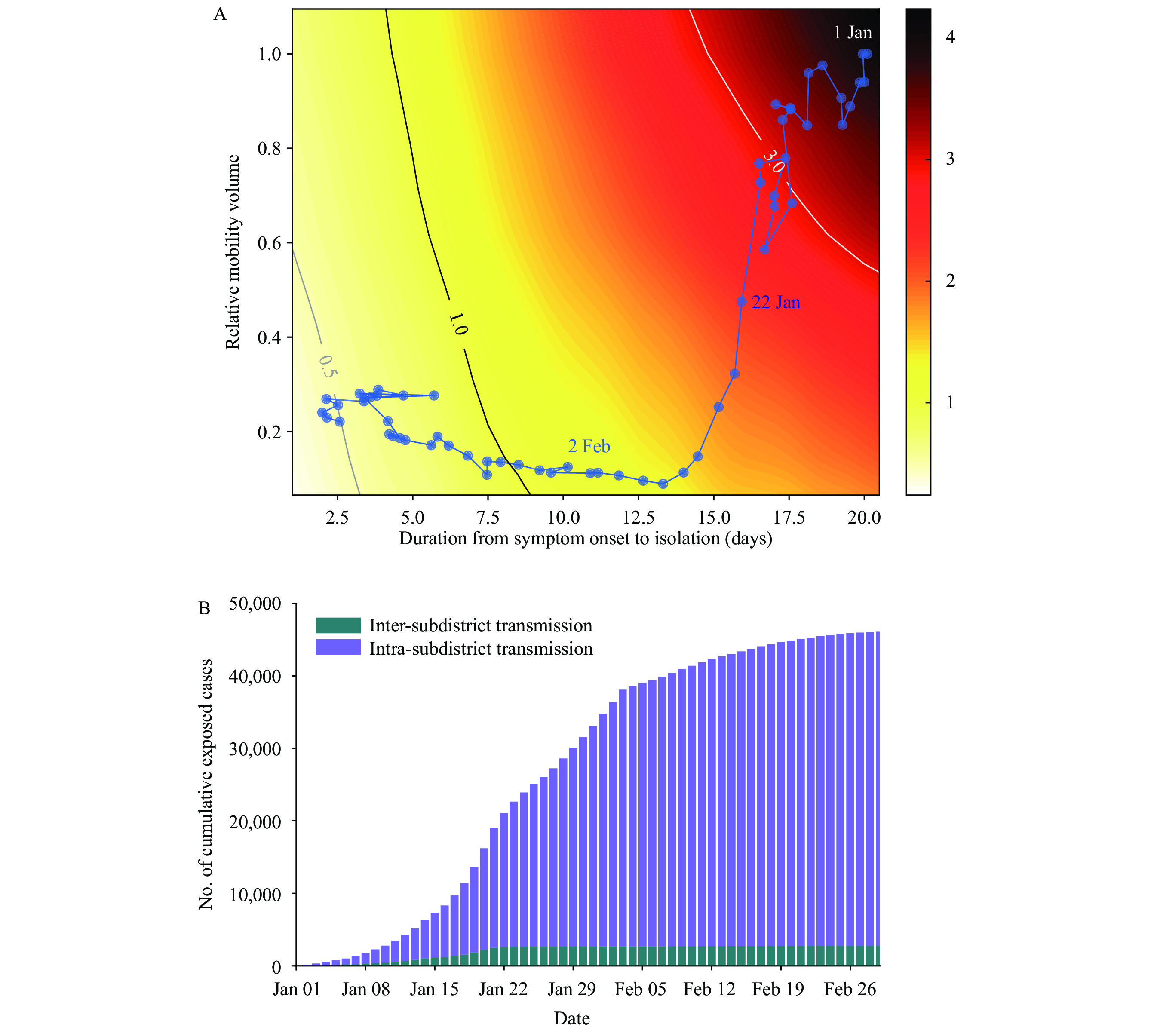

Figure 1. 

Simulation experiments on transmission dynamics and non-pharmaceutical interventions from January 1 to February 29, 2020 in Wuhan, China. (A)The contour plot between effective reproduction number $ {R}_{e} $ and the two categories of interventions implemented. (B) The number of cumulative exposed cases caused by intra- and inter-subdistrict transmissions.

Note: two categories of interventions implemented in Wuhan included mobility restriction (corresponding to relative mobility volume) and infectious period reduction (corresponding to duration from symptom onset to isolation). The color on the contour plot represents the value of $ {R}_{e} $ of corresponding relative mobility volume and duration from symptom onset to isolation. The line formed by blue dots reflects the $ {R}_{e} $ from January 1 to February 29, 2020.

We designed two scenarios to evaluate the effectiveness of non-pharmaceutical interventions. In the first scenario, we set the mobility volume after the Wuhan lockdown to the same level as the last day before the lockdown (January 22, 2020), while the infectious period is reduced to reflect reality. This scenario aims to simulate the condition where only interventions to reduce the infectious period are implemented (Scenario 1). Alternatively, in Scenario 2, we simulate the condition where only the intra-city mobility restriction is implemented. In this scenario, the duration from symptom onset to isolation after the Wuhan lockdown was set as 15.7 days (the average time on January 22, 2020) and the mobility volume was reduced to its lowest level.

We re-conducted experiments in Figure 1A with the parameters from Zhang et al. (10) to simulate the impact of the COVID-19 Delta variant B.1.617.2. Specifically, the incubation period was uniformly set to 4.4 days, and all the transmission rates were set to twice those fitted by the data. Supplementary Figure S3 showed the contour plot of $ {R}_{e} $ under the Delta variant.

We first analyzed the intra-city human mobility and transmission dynamics using a multi-phase framework. The first wave of COVID-19 in Wuhan can be divided into three phases: 1) From January 1 to January 23, 2020, there were nearly no interventions; 2) On January 23, 2020, mobility restrictions were implemented; and 3) On February 3, 2020, in addition to mobility restrictions, large-scale centralized isolation policies for suspected, mild patients, and close contacts were implemented to reduce the duration of the infectious period (11).

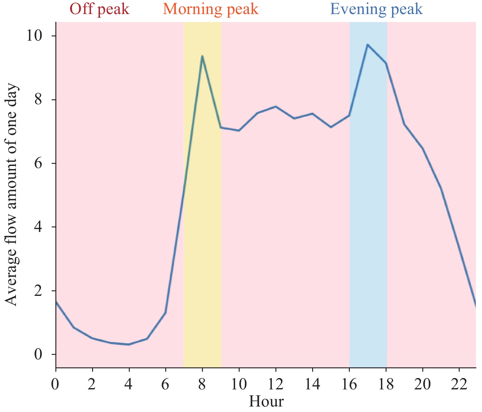
Based on the above framework, we further analyzed the role of resident mobility in intra- and inter-subdistrict transmission. We used the mobility network measured by cell phone data to establish a metapopulation model to simulate the spread of the disease within and between subdistricts (Supplementary Material and Supplementary Figure S1). Since different travel purposes may lead to different behaviors that could impact transmission, we further divided residents’ inter-subdistrict mobility into three categories based on the hours of a day (Supplementary Figure S2C and Supplementary Figure S4): the morning-peak period (7 a.m. to 9 a.m.), the evening-peak period (4 p.m. to 6 p.m.), and the off-peak period (the remaining hours of the day). Therefore, in our model, the infection rate of a contact is determined by subdistricts, mobility type (intra- and inter-subdistrict), and mobility purpose (during morning-peak, evening-peak, and off-peak periods). Our model accurately captured the daily number of onset cases in all 99 subdistricts, with a mean absolute percentage error (MAPE) of 7.04% (see Supplementary Figures S5 and S6). We investigated the influence of intra- and inter-subdistrict mobility on COVID-19 transmission using the model. Before intra-city mobility was restricted, the volume of intra- and inter-subdistrict mobility was 71.9% and 28.1%, respectively. This indicates that intra-subdistrict mobility was about 2.5 times higher than inter-subdistrict mobility. Our model indicated that the number of infections caused by intra-subdistrict transmission in the first phase was 20,011 [95% confidence interval (CI): 18,556–21,967], which was approximately 7.6 times (95% CI: 6.9–8.4) that caused by inter-subdistrict transmission (2,650, 95% CI: 2,209–3,164).

We analyzed the relationship between inter- and intra-subdistrict transmission. In the second phase, the inter-subdistrict mobility was suppressed by 98.9% due to mobility restrictions (Figure 2), resulting in almost complete termination of the inter-subdistrict transmission (Figure 1B). The intra-subdistrict mobility decreased by 84.0% (Figure 2), yet the intra-subdistrict transmission persisted until the centralized isolation policy was implemented (Figure 1B). Our model showed that the intra-subdistrict transmission caused 23,321 (95% CI: 21,097–25,350) infections after the mobility restrictions, accounting for 99.5% (95% CI: 99.5%–99.5%) of the new infections. According to individual-level clinical data, the average time from onset to isolation of a case was more than 15 days in the first phase, reducing to less than 3 days in the third phase (Supplementary Figure S2).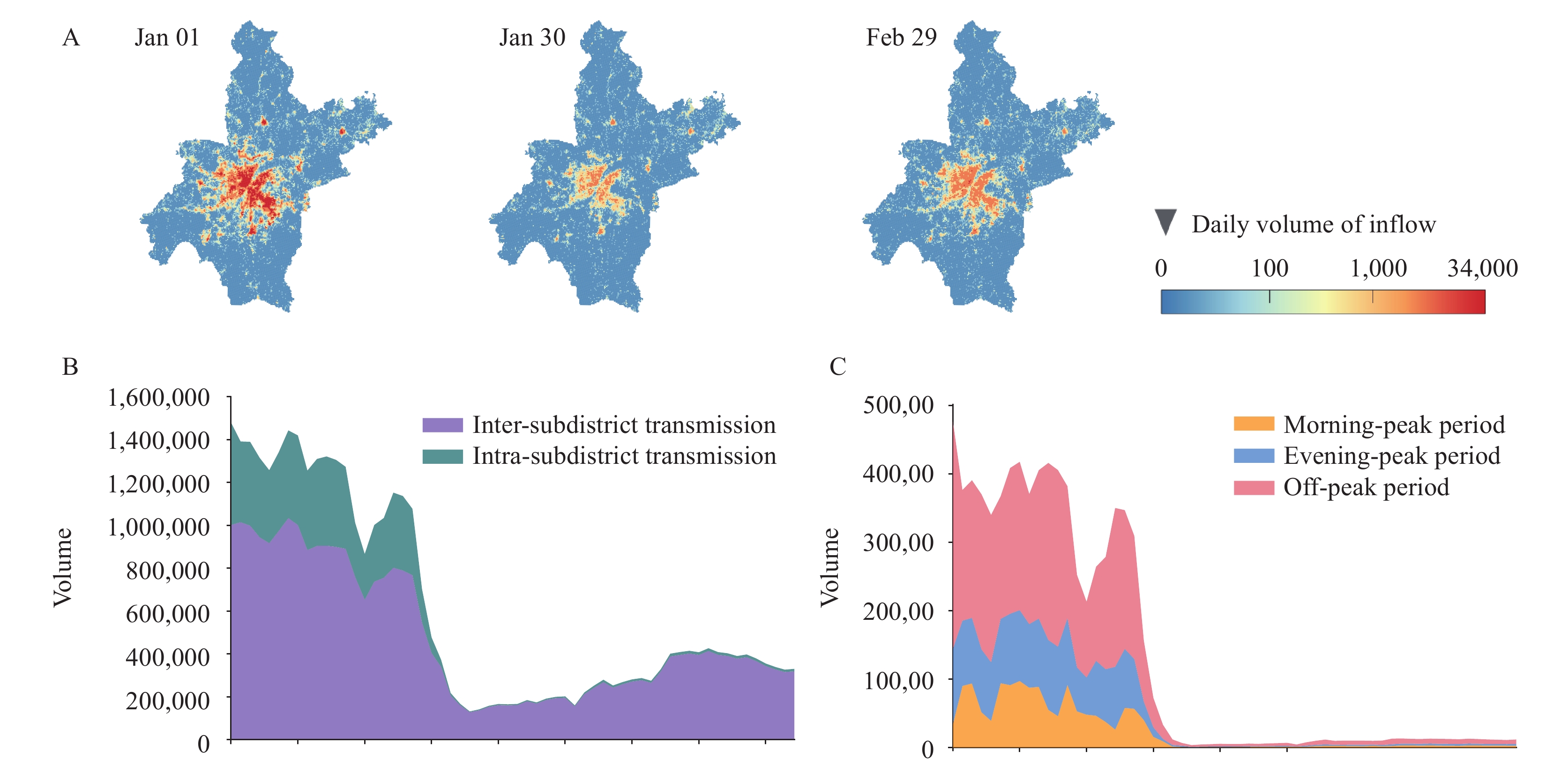

Figure 2. 

Dynamics of intra-city mobility from January 1 to February 29, 2020 in Wuhan, China. (A) The heatmaps of average daily inflow mobility volume for each subdistrict in Wuhan with different dates among the three phases. (B) Changes of intra- and inter-subdistrict mobility volume in Wuhan during the outbreak. (C) Changes of inter-subdistrict mobility during different peak periods of one day.

Since 2021, the COVID-19 Delta variant B.1.617.2 has spread rapidly around the world, posing a serious challenge to containing the pandemic. We designed a scenario to simulate the case of the Delta variant transmitting in Wuhan in early 2020, and investigated the impacts of the interventions discussed above using parameters obtained from Zhang et al. (10) (Supplementary Material). Under this scenario, mobility restriction alone is unable to reduce $ {R}_{e} $ to 1 due to the high transmissibility of the Delta variant, and containment of the epidemic could only be achieved by a 30% relative mobility volume, together with a short infectious period (less than 2.5 days) (Supplementary Figure S3). There would be an estimated 3.81 million (95% CI: 3.54–4.02 million) cases as of March 1, 2020, if the same interventions were implemented in Wuhan under the Delta variant. This result indicates the difficulty of containing this new variant, and underscores the importance of reducing the infectious period.

Our work also investigated the effectiveness of non-pharmaceutical interventions implemented in Wuhan. Although travel restrictions could reduce the number of new cases in the short term, they were not sufficient to terminate transmission. Strict isolation policies in exchange for a relaxation of traffic control have been helpful in restoring the economy damaged by the epidemic. In fact, this was the policy that the Chinese government adopted to reduce the spread of the virus. During several rounds of cluster outbreaks after May 2020 in China, the government blocked communities and buildings with confirmed cases, implemented large-scale nucleic acid tests, and enforced strict isolation policies to reduce the duration of the infection (12-13). Comprehensive and precise control measures can contain the outbreak while minimizing its impact on people’s daily lives and the economy.

In summary, we completed a review of the Wuhan COVID-19 outbreak using a refined metapopulation model. Based on this, we can make counterfactual inferences about policies that are more beneficial for decision-making in advance than the predictions and analyses of similar work (10,14).

However, the metapopulation model used in this work has limitations in terms of generalizability. First, this model requires high-quality raw data and refined population flow data. Second, the number of parameters is large, and when the preset parameters are significantly different from the original data, effective fitting cannot be achieved.

No conflicts of interest.

The epidemiological data of Wuhan were extracted from the Notifiable Disease Report System of China. This study used anonymous individual coronavirus disease 2019 (COVID-19) case data, including residential subdistrict, date of onset, and date of confirmation, from January 1, 2020 to March 1, 2020, for analysis. The demographic data for the subdistricts in Wuhan City, including population and geographical boundaries, were obtained from the Sixth Census conducted by the National Bureau of Statistics. We matched the epidemiological cases to the subdistricts. A total of 161 subdistricts with COVID-19 cases were used for further analysis. Since there were subdistricts with insufficient cases of COVID-19 to be modeled, we merged the epidemiological and demographic data of these subdistricts into the geographically closest subdistricts. Lastly, there are n=99 subdistricts for model simulation.

We used cell phone signaling data as a proxy to measure population mobility in Wuhan during the epidemic. The anonymous cell phone mobility data, provided by a major mobile carrier in China, covered approximately 51.9% (5.82 million/11.21 million) of the population in Wuhan. The raw cell phone signaling data records the visiting trajectories of cell phone users at each cellular base station. We integrated the raw data as travel flow of phone users between 500 m $ \times $ 500 m grids for each hour. We further integrated the data as travel flow between subdistricts by merging the flows of grids in the same subdistrict together.

Supplementary Figure S4 illustrates the average hourly volume of inter-subdistrict mobility on workdays prior to January 23, 2020. As shown in the figure, there is a morning peak at 8 a.m. and an evening peak at 5 p.m., reflecting the temporal rhythm pattern of residents’ mobility behaviors on workdays. Based on this, we classified residential mobility in one day into three categories based on the time of departure. The first category is the mobility from 7 a.m. to 9 a.m., i.e., the morning rush hour when people commute to work from their homes. The second category is the mobility from 4 p.m. to 6 p.m., i.e., the evening peak period when people are returning home from their workplaces. The last one is mobility during off-peak periods, excluding morning and evening rush hours. The mobility during the off-peak period is relatively random.

In order to study the impacts of different patterns of resident mobility on intra-city epidemic transmission, our model refines the transmission process into two parts, namely the intra-subdistrict transmission and the inter-subdistrict transmission, and further divides the inter-subdistrict transmission into three categories, i.e., transmission in the evening-peak, morning-peak, and off-peak periods. As shown in Formula 1, for the intra-subdistrict transmission, the number of newly exposed population for metapopulation i in one day is $ \beta \dfrac{{S}_{i}}{{N}_{i}}{I}_{i} $, which is the same as the definition of the standard SEIR model. For the inter-subdistrict transmission, the increment of the exposed population in the metapopulation i caused by the inflow mobility from the metapopulation j is expressed as $ \beta \dfrac{{S}_{i}}{{N}_{i}}{I}_{j2i} $, where $ {I}_{j2i} $=$ \dfrac{{T}_{hjit}\cdot {C}_{j}}{{N}_{j}}{I}_{j} $, i.e., the infectious population traveled from the metapopulation j to i, is calculated using $ {I}_{j} $ and scaled by human mobility data. Here, $ {N}_{j} $ represents the population of subdistrict $ j $, which is obtained from the census data. $ {T}_{hjit} $ is the amount of inter-subdistrict mobility from the subdistrict $ j $ to $ i $ in the period $ h $ of the day t, where h=1 for the morning-peak, h=2 for the evening-peak, and h=3 for the off-peak period. The parameter $ {C}_{i} $ the ratio of $ {N}_{i} $ and the number of cell phone users in subdistrict i, which is used to calibrate the mismatch between cell phone users and the population.

As different patterns of mobility should have different effects to transmission of COVID-19, we set the transmission rate $ \beta $ as four types in Formula 1. Specifically, $ {\beta }_{\mathrm{1,1}}^{i} $, $ {\beta }_{\mathrm{1,2}}^{i} $, $ {\beta }_{\mathrm{1,3}}^{i} $ denote the transmission rates for the inter-subdistrict transmission in the evening-peak, morning-peak, and off-peak periods in the metapopulation i, respectively, while $ {\beta }_{2}^{i} $ denotes the transmission rate of intra-subdistrict transmissions in the metapopulation i. The presymptomatic infectious population may have different infectiousness with infectious population (1), we multiply $ \beta $ with a factor q for the transmission between presymptomatic infectious population and susceptible population.

In the epidemiological data, the original record of each infected case includes two dates: the date of symptom onset and the date of laboratory confirmation. We sampled an incubation period from a Weibull distribution, as reported in a previous study (2). By using the sampled incubation period and the symptomatic onset date, we can approximate the exposure date for each case. Moreover, we set the last 2.3 days of the incubation period as the presymptomatic infectious period according to previous studies (3). In this way, the timeline for an infected case is divided as five periods, i.e., the Susceptible period (before the date of exposure), the Exposed period (from the date of exposure to 2.3 days before the date of onset), the Presymptomatic infectious periods (the last 2.3 days before the date of onset), the Infectious periods (from the date of onset to the date of confirmation), and the Removal periods (after the date of confirmation). We set a confirmed case as a removed one since all infected persons will be immediately quarantined once they get confirmation in China and therefore would not cause secondary infections anymore. We calculate the size of population $ {E}_{i} $, $ {P}_{i} $, $ {I}_{i} $ $ {R}_{i} $ in Formula (1) using the number of cases on each day for each subdistrict i, and calculate the size of the susceptible population as $ {S}_{i}={N}_{i}-{E}_{i}-{P}_{i}-{I}_{i}-{R}_{i} $.

In Formula (1), the transition rate $ {\alpha }_{e} $ is set as the inverse of the average period between exposure and presymptomatic infectious (the incubation period minus 2.3 days), and the incidence rate $ {\alpha }_{p} $ is set as the inverse of the average presymptomatic infectious period (2.3 days). The removal rate $ \gamma $ is dynamically set as the inverse of the average duration from symptom onset to confirmation for every day. As shown in Supplementary Figure S2, this duration substantially reduces as a result of intervention policies.

In our model, we set the transmission rates $ \beta $ in a dynamic way. Given a subdistrict i, there are four transmission rates, namely $ {\beta }_{\mathrm{1,1}}^{i} $, $ {\beta }_{\mathrm{1,2}}^{i} $, $ {\beta }_{\mathrm{1,3}}^{i} $, $ {\beta }_{2}^{i} $. For any one of the four transmission rates, denoted as $ {\beta }_{*}^{i} $, we set it as $ {\beta }_{*}^{i}={\widehat{\beta }}_{*}^{i}\cdot {M}_{t}^{i} $ on the day t, where $ {\widehat{\beta }}_{*}^{i} $ is a basic transmission rate and $ {M}_{t}^{i} $ is the total volume of resident mobility in the subdistrict i on the day t. The $ {M}_{t}^{i} $ is calculated as $ {M}_{t}^{i}=\dfrac{{\sum }_{ij}^{}{w}_{ijt}+{h}_{ijt}+{r}_{ijt}}{{N}_{i}} $, where $ {w}_{ijt} $ is the amount of inter-subdistrict mobility from subdistrict i to subdistrict j during the morning-peak (to-workplace) period, $ {h}_{ijt} $ is during the evening-peak (to-home) period, and $ {r}_{ijt} $ is during the off-peak period.

The basic transmission rates $ {\widehat{\beta }}_{\mathrm{1,1}}^{i} $, $ {\widehat{\beta }}_{\mathrm{1,2}}^{i} $, $ {\widehat{\beta }}_{\mathrm{1,3}}^{i} $, $ {\widehat{\beta }}_{2}^{i} $, and the presymptomatic infectiousness discount factor q are calibrated by the Metropolis-Hastings Markov Chain Monte Carlo (MCMC) algorithm (4), with the state $ {P}_{i} $, $ {I}_{i} $ $ {R}_{i} $ for each day as supervisions. The process of the parameter generation is performed separately for each subdistrict and for three phases. For each phase, after a burn-in of 1,000 iterations, we run the MCMC simulation for 10,000 times, with sampling at every 50th step. The average root mean square error (RMSE) for each subdistrict is 4.35, and the simulation results are shown in Supplementary Figure S5. The calibration of parameters is performed with the Python (version 3.6.0, Python Software Foundation, Wilmington, US) and the Python package PyMC (version 2.3.8) (5).

We derive the effective reproduce number $ {R}_{e} $ of the metapopulation SEPIR model by the next generation matrix (6). Suppose a model with $ m $ metapopulations, let $ x={\left({E}_{1},{E}_{2},\dots ,{E}_{m},{P}_{1},{P}_{2},\dots ,{P}_{m},{I}_{1},{I}_{2},\dots ,{I}_{m}\right)}^{T} $ be the number of individuals for each infected compartments, ${u}_{i}=\dfrac{{S}_{i}}{{N}_{i}}{\beta }_{2,1}^{i},{v}_{ji}={\sum }_{h}^{}{\beta }_{1,h}^{i}\dfrac{{S}_{i}}{{N}_{i}}\dfrac{{T}_{hji}}{{N}_{j}}{c}_{j}.$

Furthermore, we have

Where $ {F}_{i}\left(x\right) $ is the rate of generating new infections in the i-th compartments of vector $ x $, $ {V}_{i}\left(x\right) $ is the transition rate of infections in the i-th compartments of vector $ x $ by all other means, $ F\left(x\right),V\left(x\right)\in {R}^{3m\times 1} $, and based on the ordinary differential equations in Formula (1), we can derive the formulation of $ F\left(x\right) $ and $ V\left(x\right) $ as

With $ {F}_{E}\left(x\right)={\left[{\sum }_{j\ne i}^{}q{v}_{ji}{P}_{j}+q{u}_{i}{P}_{i}+{\sum }_{j\ne i}^{}{v}_{ji}{I}_{j}+{u}_{i}{I}_{i}\right]}_{i=1}^{m},{F}_{P}\left(x\right)={F}_{I}\left(x\right)={O}^{m\times 1} $,

With $ {V}_{E}\left(x\right)={\left[{\alpha }_{e}{E}_{i}\right]}_{i=1}^{m},{V}_{P}\left(x\right)={\left[-{\alpha }_{e}{E}_{i}+{\alpha }_{p}{P}_{i}\right]}_{i=1}^{m},{V}_{I}\left(x\right)={\left[-{\alpha }_{p}{P}_{i}+\gamma {I}_{i}\right]}_{i=1}^{m}. $

Next, we have the matrix

Where $\left[\dfrac{\partial {F}_{E}^{i}\left(x\right)}{\partial {P}_{j}}\right]=\{q{u}_{i},i=jq{v}_{ji},i\ne j,\left[\dfrac{\partial {F}_{E}^{i}\left(x\right)}{\partial {I}_{j}}\right]=\{{u}_{i},i=j{v}_{ji},i\ne j$, and other sub-matrixes are $ {O}^{m\times m} $.

Similarly, we have

and

Where $ 1 $ denotes identity matrix.

Based on this, we can derive the next generation matrix for the metapopulation SEPIR model as

Where $ A=\{\dfrac{q{u}_{i}}{{\alpha }_{p}}+\dfrac{{u}_{i}}{\gamma },i=j\dfrac{q{v}_{ji}}{{\alpha }_{p}}+\dfrac{{v}_{ji}}{\gamma },i\ne j,B=\{\dfrac{q{u}_{i}}{{\alpha }_{p}}+\dfrac{{u}_{i}}{\gamma },i=j\dfrac{q{v}_{ji}}{{\alpha }_{p}}+\dfrac{{v}_{ji}}{\gamma },i\ne j,C=\{\dfrac{{u}_{i}}{\gamma },i=j\dfrac{{v}_{ji}}{\gamma },i\ne j $, and other sub-matrixes equal to $ {O}^{m\times m} $.

Finally, by Driessche and Watmough (6), the effective reproduce number $ {R}_{e} $ can be derived as

Where $ \rho \left(A\right) $ represents the spectral radius of a matrix $ A $. According to the property of matrix computation, this is equivalent to the maximum of absolute eigenvalues of the matrix

We adjust the parameters of the calibrated model to estimate the effectiveness of different interventions and their interactions to the effective reproduce number $ {R}_{e} $. Using the calibrated model parameters on January 23, 2020 as the benchmark, we adjust the resident mobility intensity, i.e., $ {w}_{ijt} $, $ {h}_{ijt} $, and $ {r}_{ijt} $, to simulate the effectiveness of the mobility restriction policy, as well as adjust the average duration from symptom onset to isolation, i.e., $\dfrac{1}{\gamma }$, to simulate the effectiveness of the infectious period reduction policies. We construct the contour plot of $ {R}_{e} $ in Figure 2 through traversing the relative resident mobility intensity and average duration from symptom onset to isolation to generate corresponding effective reproduction numbers.

We design two scenarios to evaluate the effectiveness of non-pharmaceutical interventions. In the first scenario, we set mobility volume after the Wuhan lockdown to be the same as the last day before the lockdown (January 22, 2020), while the infectious period declines as the reality. This scenario is set to simulate the condition where only the interventions to reduce the infectious period are implemented, which is called Scenario 1. Oppositely, in the second scenario (Scenario 2), we simulate the condition where only the intra-city mobility restriction is implemented, where the duration from symptom onset to isolation after the Wuhan lockdown is set as 15.7 days (the average time on January 22, 2020) in the model, and the mobility volume drops to its lowest level as the reality.

To simulate the impact of the COVID-19 Delta variant B.1.617.2, we reconducted the experiments in Figure 2 with the parameters from Zhang et al. (7). Specifically, the incubation period was set to 4.4 days uniformly, and all the transmission rates were set to 2 times of those fitted by data. Supplementary Figure S3 shows the contour plot of $ {R}_{e} $ under the Delta variant.

He X, Lau EHY, Wu P, Deng XL, Wang J, Hao XX, et al. Temporal dynamics in viral shedding and transmissibility of COVID-19. Nat Med 2020;26(5):672 − 5. http://dx.doi.org/10.1038/s41591-020-0869-5. Backer JA, Klinkenberg D, Wallinga J. Incubation period of 2019 novel coronavirus (2019-nCoV) infections among travellers from Wuhan, China, 20-28 January 2020. Euro Surveill 2020;25(5):2000062. http://dx.doi.org/10.2807/1560-7917.ES.2020.25.5.2000062. Hao XJ, Cheng SS, Wu DG, Wu TC, Lin XH, Wang CL. Reconstruction of the full transmission dynamics of COVID-19 in Wuhan. Nature 2020;584(7821):420 − 4. http://dx.doi.org/10.1038/s41586-020-2554-8. Haario H, Saksman E, Tamminen J. An adaptive Metropolis algorithm. Bernoulli 2001;7(2):223 − 42. http://dx.doi.org/10.2307/3318737. Patil A, Huard D, Fonnesbeck CJ. PyMC: Bayesian stochastic modelling in python. J Stat Softw 2010;35(4):1-81. https://pubmed.ncbi.nlm.nih.gov/21603108/. van den Driessche P, Watmough J. Reproduction numbers and sub-threshold endemic equilibria for compartmental models of disease transmission. Math Biosci 2002;180(1 − 2):29 − 48. http://dx.doi.org/10.1016/S0025-5564(02)00108-6. Zhang M, Xiao JP, Deng AP, Zhang YT, Zhuang YL, Hu T, et al. Transmission dynamics of an outbreak of the COVID-19 Delta variant B.1.617.2 — Guangdong province, China, May–June 2021. China CDC Wkly 2021;3(27):584-6. http://dx.doi.org/10.46234/ccdcw2021.148.